Images and other media content are becoming a predominant part of data in 21st century due to the rise of smartphones and the ease at which pictures can be taken nowadays. Images are also becoming common in other domains such as medical, engineering etc. Therefore it becomes important for us to understand the nature of these digital images and how to address them in a deep learning domain.

Nature of Digital Images

Digital Images can often be described as mere rectangular collection of pixels. Each of these pixels store a color represented using the RGB Model. Each pixel in an image has a color code similar to those in Table 1 with each of RGB taking a value between 0 and 255. An accumulation of 1000×1000 such pixels make up a image of size 1 megapixel.

Color Name	Hex Code	RGB Values
White	FFFFFF	(255,255,255)
Black	000000	(0,0,0)
Red	FF0000	(255,0,0)
Green	00FF00	(0,255,0)
Blue	0000FF	(0,0,255)

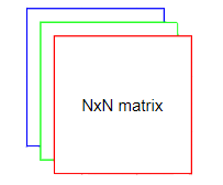
Now we separate this into three different channel for each color (RGB). This means for representing a 1000×1000 pixel image we need three 1000×1000 matrices with each element containing a value between 0 and 255. By convention we take first 1000×1000 matrix as the values of red, second as green and third as blue. We can see that the matrix can be represented as 1000x1000x3 where three denotes the number of channels.

Convolution Operation

Convolution Operation in mathematics is an operation between two functions which produces a third function, which depicts the affect of one function on the shape of the other. The same logic is going to be used in convolutional neural networks where we have a filter of size fxf (referred to as kernel) which is convoluted on the image matrix of size NxN.

Note: In mathematics while performing convolution operation, we transpose and shift the second function, however this is not done in deep learning. The convolution operation in deep learning is equivalent to cross-correlation in mathematics.

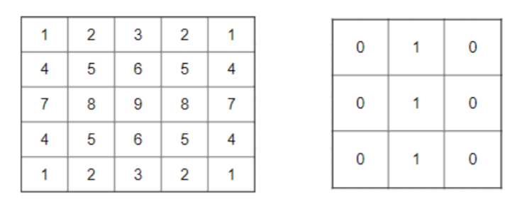
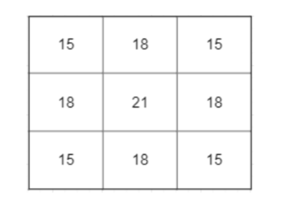
Let us consider the matrices in Figure 2. Using the 3×3 filter we can perform convolution over our image. Let us consider the first 3×3 sub-matrix present in our image [[1,2,3],[4,5,6],[7,8,9]]. Performing convolution using our filter we will get output as 15. Similarly when we do convolution over the rest of the image we will get the following matrix as output.

In a convolutional neural network, we have many such filters which learn to identify features from the images. If we have n filters in a layer then the output will have n convolved matrices stacked together. The size of convolved image for a filter of size fxf and image of size NxN can be found using the following equation

Padding

Padding refers to process of adding a border to the image matrix (generally filled with 0’s) so that the Output Matrix of convolution operation does not shrink and the corner elements are given equal importance. The number of borders to be added to the image is determined by its hyper parameter. Figure 4 shows a simple 3×3 image matrix that is padded symmetrically with padding = 1.

From the Figure 4 we can see that on padding symmetrically, the dimensions of padded matrix increases by 2 * pad in height and width. Therefore in output matrix equation, image matrix NxN will now be (N+ 2 * pad) x (N + 2 * pad). Therefore we can rewrite the dimension of Output Matrix as as:

If we perform convolution operation on the padded matrix in Figure 4, with filter of size 3×3, we see that the resultant matrix will be of size 3×3 which is the same as dimension as the image matrix. Such padding value where the Output Matrix on convolution has the same size as the image matrix is called “same” padding. From a given filter size f we can find the padding required pad using above equation. The pad value for “same” padding for a given filter size f will be:

Stride

Stride is another common hyperparameter associated with convolution operation. It refers to the number of steps to be taken while performing convolution operation. In Figure 5 we can see that the first convolution is done at index (0,0) while the second convolution is done at (0,2). This is because the stride is 2 in this case and therefore it jumps by two while considering the next matrix for convolution. Similar pattern is followed while shifting rows therefore after (0,2) the next index will be (2,0).

Stride operation helps in reducing the computation time of convolution by reducing the number of submatrix considered from the image. This also will impact the size of Output Matrix as the dimensions of Output Matrix corresponds to the number of number of submatrix considered in Image. Therefore Output Matrix equation, along with strides can be rewritten as:

Convolution Layer

Convolution Layer makes up the most important part of CNNs. Convolution Layer generally haven filters of size fxf which are used to perform convolution operation on the information in the preceding layer. Let us consider NxNxc be the dimension of the input layer. Then we need filters of dimension fxfxc to perform convolution operation. If we have n’ such filter present in the layer then the number weights to be computed will be fxfxcxn’. Apart from this we are need to compute bias for each filter, therefore we will be computing n’ biases.

It must be noted that the features detected by these filters are learnt while training the network and therefore the filter matrix are initially randomly assigned and over epochs these filter start learning a particular feature from the dataset provided to it. The filters in initial layers of a CNN tend to detect simple features such as edges. However as we go deeper into the network it can detect more complex features in the image. The total number of parameters in a convolution layer can be expressed as:

In the next week’s post we will discuss the implementation of simple convolutional neural network to classify images present in Fashion MINST data, using Keras.