In the last week’s post we discussed the theoretical aspects of Convolution Operation. Today we are going to discuss the need for convolutional neural networks and its implementation for classification of fashionMNIST dataset.

Need for CNNs

A normal Artificial Neural Network architecture often fails when dealing with Image based dataset mainly because of the humongous amount of parameters required, to even form a shallow neural network.

Let us consider an example where we have a dataset with images of dimension 100x100x3 to be classified as dog or not dog. To feed this as input to the neural network, we will require 30,000 nodes and let us assume we have two hidden layers with 160,000 and 320,000 neurons. This will mean that for a fully connected network, the number of parameters between input layer and 1st hidden layer will be 30,000 * 160,000 + 160,000, which is 4,800,160,000 parameters! The overall parameters for the above mentioned architecture will be fifty-six billion eight hundred thousand one! This makes it really hard to train a deep artificial neural network on image based datasets.

On the other hand, convolutional neural networks are able to process the same image but with lesser amount of parameters because of two main reasons:

Parameter Sharing: Convolution Neural Networks use filters as feature detectors and assumes that a detector that is useful in one part of the image will be useful in another part.

Sparsity of Connections: In a Convolutional Neural Network, each element in the Output Matrix of a convolution layer is decided by only a set of elements in the previous layer and does not require the knowledge of all other elements.

Convolutional neural networks also help maintaining the spatial information of the pixels in the image.

Figure 1. A simple Convolutional Neural Network Architecture.

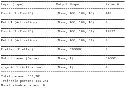
Let us consider a simple CNN architecture as shown in Figure 1. We first perform convolution operation on our 100x100x3 input image with same padding and filter of size 3×3. Let us say we have 16 such filters therefore the output of this layer will be of shape 100x100x16 which is 160,000 same as the first hidden layer in ANN. Next we perform a convolution operation with same padding and filter of size 5×5. We have 32 such filters therefore the output of this layer will be of shape 100x100x32 which is 320,000.

Now we flatten the output and connect it to a single node output layer. The number of parameters in this basic architecture will be 3x3x3x16 + 1×16 for first convolution layer and 5x5x16x32+1×32 for second convolution layer and 320,001 for final fully connected layer. The total parameter therefore for this architecture will be 333,281. This is significantly less than that of an ANN and therefore it is possible to go deeper with a CNN than with ANN.

Classification of FasionMNIST Data

Fashion-MNIST is a dataset of Zalando’s article images—consisting of a training set of 60,000 examples and a test set of 10,000 examples. Each example is a 28×28 grayscale image, associated with a label from 10 classes. We intend Fashion-MNIST to serve as a direct drop-in replacement for the original MNIST dataset for benchmarking machine learning algorithms. It shares the same image size and structure of training and testing splits.

We are now going to implement a simple CNN architecture to classify the images present in Fashion-MNIST dataset. First we need to import the dataset, and we are going to do this using Keras Framework.

import numpy as np
from keras import datasets
(x_train,y_train),(x_test,y_test) = datasets.fashion_mnist.load_data()

Next we need to format the data in a way which can be easily processed. As the images are grayscale they are two dimensional (28 x 28), however we are going to reshape it to (28 x 28 x 1) so that we can make our architecture more generic (as color images are of 3 dimensional). The label arrays have values between 0-9 with each integer denoting a different item. We need to convert this into binary class matrix using to_categorical function.

from keras.utils import to_categorical
X_train = np.reshape(x_train,(x_train.shape[0],x_train.shape[1],x_train.shape[2],1))
X_test = np.reshape(x_test,(x_test.shape[0],x_test.shape[1],x_test.shape[2],1))
Y_train = to_categorical(y_train,10)
Y_test = to_categorical(y_test,10)
print("X Train shape is:",X_train.shape)
print("Y Train shape is:",Y_train.shape)
print("X Test shape is:",X_test.shape)
print("Y Test shape is:",Y_test.shape)

Let us now import the necessary layers for our CNN Architecture.

from keras.layers import Input,Dense,Conv2D,MaxPooling2D,BatchNormalization,Flatten
from keras import Sequential

Next we will define our architecture. We are going to define a function to define our model. We’ll be using categorical crossentropy function for loss and Adam optimizer as shown below.

def create_model(input_shape,no_of_classes):
  model = Sequential()
  model.add(Input(input_shape))
  model.add(Conv2D(128,kernel_size=(3,3), activation="relu"))
  model.add(MaxPooling2D())
  model.add(BatchNormalization())
  model.add(Conv2D(256,kernel_size=(3,3), activation="relu"))
  model.add(MaxPooling2D())
  model.add(BatchNormalization())
  model.add(Conv2D(512,kernel_size=(3,3), activation="relu"))
  model.add(MaxPooling2D())
  model.add(BatchNormalization())
  model.add(Flatten())
  model.add(Dense(1024,activation="relu"))
  model.add(Dense(1024,activation="relu"))
  model.add(Dense(no_of_classes,activation="softmax"))
  return model
model = create_model(X_train[0].shape,10)
model.compile(optimizer='adam', loss='categorical_crossentropy',metrics="accuracy")
model.summary()

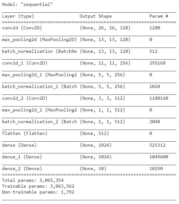
Figure 2. shows the expected output for the above code. This is the architecture we are going to train for classifying the Fashion MNIST data.

Figure 2. CNN architecture we have implemented.

We can now train our model on Fashion-MNIST dataset. We are going train it initially over 10 epochs however you can choose to train it over more.

history = model.fit(X_train,Y_train,batch_size=64,epochs=10,validation_split=0.2)

Once we are done training the model to a satisfactory accuracy, we can evaluate how the model performs on the testing data.

y_pred = model.predict(X_test)
y_pred = np.where(y_pred > 0.5, 1, 0)
print(y_pred.shape)
from sklearn.metrics import confusion_matrix
cf_matrix = confusion_matrix(Y_test.argmax(axis=1),y_pred.argmax(axis=1),normalize='true')*100
import seaborn as sns
ax = sns.heatmap(cf_matrix, annot=True,cmap="YlGnBu")
ax.set(title="Confusion Matrix",
      xlabel="True Value",
      ylabel="Prediction",)
sns.set(font_scale=1)

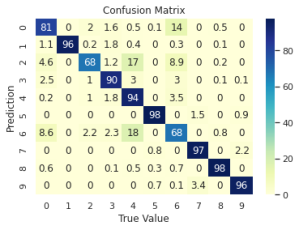
In the above code snippet we have depicted the performance of our model using confusing matrix as showing in Figure 3.

Figure 3. Performance of model on testing data.

You can find the code for this blogpost in this github repo.