Many real life scenarios generate sequential data, where the details of the preceding states play an important role in determining the outcome of the current state. Examples of sequential data are DNA Sequence, Text Documents, Stock prices etc. In such cases, the output of a particular state, will not only depend on the input provided but also the previous states encountered by our model.

Let us consider the example of Natural Language Translation. While we could have a lookup table that translates the sentence provided word-by-word into another language, this will lose the grammatical structure and in many cases the meaning the original sentence was trying to convey. This is because in a word by word model, rather than understanding the meaning of the words with respect to the context they appear in, we are just translating it to an equivalent word from our desired output language.

On the other hand, literal translation understands the meaning of the word or phrase with respect to the context they appear in and then translates it to our desired output language. This plays an important role when dealing with idioms, ambiguous words etc. which cannot be directly mapped to a word or phrase in another language. This is where RNN-like architecture comes into picture, where we process the sequence as a whole.

Figure 1. Diagram of different RNN sequence types. Credit: Andrej Karpathy

Introduction to RNN

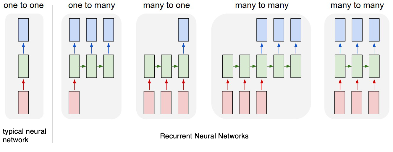
RNN stands for Recurrent Neural Networks, which is a class of artificial neural networks where there exists a connection between nodes, forming a directed graph along the temporal sequence. This means the network, while might take input in a particular state, will also use the state in the node/neuron was in the previous iterations. This way, we are able to analyze sequence of data which are related to each other.

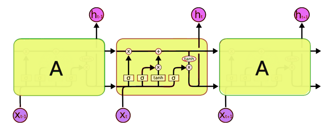
One of the common and most successful RNN architecture is called LSTM (Long Short Term Memory) whose architecture has been depicted in Figure 2. The various gates that are present in a common LSTM architecture has been explained in detail in this particular blogpost.

Figure 2. LSTM Architecture Credits Analytics Vidhya

Sentiment Analysis Using RNN

Let us now try developing a model for sentiment analysis on twitter samples dataset, we considered in the previous blogpost. We are doing so that we can make a comparison between both the methodologies and see which works better for this particular use case. After importing and preprocessing the twitter samples corpus, we are going to identify how often does a word occur in positive tweets and negative tweets. The positive and negative frequency thus found will act as the features for our RNN Model.

Using the positive and negative counts of words, we are going to present the tweets as a Nx2 matrix, with the first column containing the positive frequency of the word and second column representing the negative frequency. The below figure, depicts the way tweets are represented in different stages.

Let us now implement an RNN using Keras, to perform sentiment analysis on the given dataset. The first step is to import the necessary function from Keras.

from keras.models import Sequential
from keras.layers import Dense, Dropout, LSTM, Reshape
from keras.optimizers import Adam

Next, we will be writing a function which will make us our RNN model using LSTM Architecture.

def create_model(inp_shape,batch_size):
    model = Sequential()
    model.add(LSTM(512, input_shape = inp_shape, activation = 'relu'))
    model.add(Dense(1024,activation='relu'))
    model.add(Dropout(0.1))
    model.add(Dense(2048,activation='relu'))
    model.add(Dropout(0.1))
    model.add(Dense(2048,activation='relu'))
    model.add(Dropout(0.1))
    model.add(Dense(1,activation='sigmoid'))
    return model
BATCH_SIZE = 32
model = create_model(X_array[0].shape,BATCH_SIZE)
model.summary()

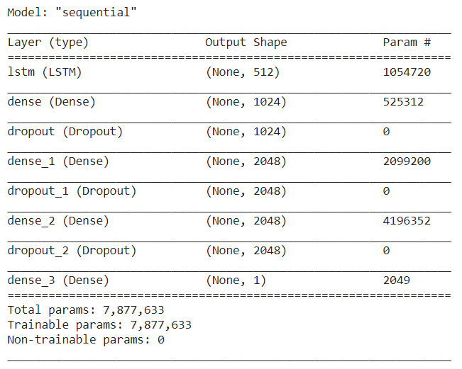
The above code generates our model which has been summarized below.

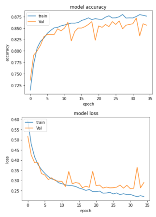
Let us now train our model, using Adam’s optimizer. We are going to use Binary Cross Entropy loss function as the output generated by our model belongs to two classes, positive or negative. Once trained, you will see that model has an accuracy of around 86% on test dataset, which is significantly better than Naive Bayes Approach.

opt = Adam(learning_rate=0.00005)
model.compile(optimizer=opt, loss='binary_crossentropy', metrics=['accuracy'])
history = model.fit(x=x_train,y=y_train,epochs=35,validation_split=0.1,batch_size=BATCH_SIZE,validation_steps=20,shuffle=True)

While accuracy of 86% is good, it can be further improved by processing the tweets better and also using concepts such as word embedding to make sure that meaning of the words is better understood. Furthermore the model implemented is simplistic and a more sophisticated model can do a better approach with the given data.

Figure 3. Accuracy and Loss of Train and Validation Data

You can find the code for this blogpost in this github repo.