Face detection is one of the most popular application of computer vision, with even the modern smartphones having face recognition based locking system. It also acts as a stepping stone to enter the domain of computer vision, which has been revolutionizing various fields from surgical procedures to self driving cars.

One of the earliest ideas behind face detection was proposed by Viola and Jones in their paper Rapid object detection using a boosted cascade of simple features, where they proposed the usage of haar-like features to determine whether a given image contains human face and if so, where.

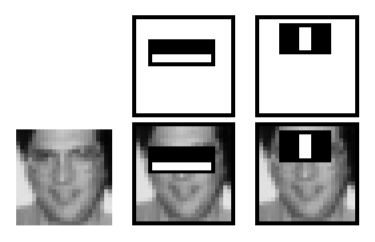
Haar-like features in Viola-Jones Algorithm are simple rectangular features that maybe present within the provided image at any position or scale. These help in determining the existence/absence of certain characteristics or pattern in the image. Figure 1, depicts a simple Haar-Like Feature which checks for rectangular blocks within the image where the bottom half is significantly brighter than the upper half.

Figure 1. A simple rectangular Haar-Like Feature

However the issue is when we consider various possible filters, even for a image of 24×24 there will be around 160000 features. For each of these feature we have to compute the sum of pixels under the brighter and darker region. To solve this, we are going to consider integral image, thus reducing the computation to mere 4 pixels.

Another thing observed in Viola-Jones Algorithm is that most of the features do not contribute much. Therefore we will be wasting resources computing the features which contribute almost nothing towards our end result. To select the best features for face detection, we consider a training dataset, some of which contain face while others don’t. Now we train all the features over the dataset, and identify which features are able to classify the images with least error (The actual algorithm used is called Adaboost). In the paper mentioned above, the authors were able to achieve 95% accuracy with mere 200 filters. The final model proposed had 6000 filters.

Figure 2. Features that are able to detect important features like eyebrows etc. (Taken for Viola Jones Paper)

Now we are able to detect a face in the image however in an image, most of the region is non-face region and therefore processing over them will be inefficient. This was addressed by the authors by introducing a cascade of classifiers, wherein instead of applying all 6000 filters together, they are divided into group of filters applied one-by-one. If a region within the image fails the very first stage, it is discarded.

The author’s final detector had 38 such stages with the first five stages having 1, 10, 25, 25 and 50 filters respectively.

Let us now try to implement the above discussed concepts using OpenCV library of python. First we’ll try to generate integral images for a given grayscale image. For this, first we’ll import the necessary libraries, which are OpenCV (cv2) and numpy.

import cv2
import numpy as np

Now, we need to import the image and identify the dimension of the image (rows and columns)

image = cv2.imread("regular_image.png")
image = cv2.cvtColor(image, cv2.COLOR_BGR2GRAY)
rows, cols = image.shape

We’ll define a numpy array filled with zeros which will act as the destination for the integral image.

dest = np.zeros((rows,cols),np.float32)

We’ll generate the integral image for the input image using OpenCV function “integral”. The image is then normalized so that we can visualize it.

integral_image = cv2.integral(image,dest,cv2.CV_32F)
cv2.normalize(integral_image, integral_image, 0, 1, cv2.NORM_MINMAX) 

Let us now print the original image and the integral image.

cv2.imshow('Original Image',image)
cv2.imshow("Integral Image",integral_image)
cv2.waitKey()

Next up, let us try to implement Haar Cascade Classifier. For this we are going to use the already trained cascades available here. We are going to be using the default frontal face cascade and the smile cascade in this example.

import numpy as np
import cv2
 
face_cascade = cv2.CascadeClassifier('haarcascade_frontalface_default.xml')
smile_cascade = cv2.CascadeClassifier('haarcascade_smile.xml')

Now that we have imported the required cascade classifiers, let us import the image we are going to test it on. The imported image is converted to grayscale.

img = cv2.imread('image.jpg')
gray = cv2.cvtColor(img, cv2.COLOR_BGR2GRAY)

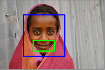
Now using the face cascade we will detect the occurrence of faces in our image, and loop through each face to check if we can detect a smile or not. We will be drawing bounding boxes around every face we identify (blue in color) and smile (green in color).

faces = face_cascade.detectMultiScale(gray)
for (x,y,w,h) in faces:
    img = cv2.rectangle(img,(x,y),(x+w,y+h),(255,0,0),2)
    roi_gray = gray[y:y+h, x:x+w]
    roi_color = img[y:y+h, x:x+w]
    smile = smile_cascade.detectMultiScale(roi_gray)
    for (sx,sy,sw,sh) in smile:
        cv2.rectangle(roi_color,(sx,sy),(sx+sw,sy+sh),(0,255,0),2)

Now let us the display the image and see how well is the image able to detect a smile.

cv2.imshow('img',img)
cv2.waitKey()

Figure 3. The output of smile detection program using OpenCV and Haar Cascade Classifier

Congrats on successfully implementing a smile detector! You can find all the codes and input files used in the blog post over here, along with a code for eye detection on webcam video: GitHub Week 1 – Smile Detection