Classification is one of the most fundamental and intuitive things that we humans do, often without even realizing it.

“Will that t-shirt look good on me or not? Is it going to rain or not?”

The human brain is naturally tuned to make such decisions however, replicating it in a computer system is not as simple. In this blogpost, we are going to talk about Support Vector Machines and how they can be used for Binary Classification of data.

Figure 1. In the above image we have datapoints belonging to two colors; blue and orange.

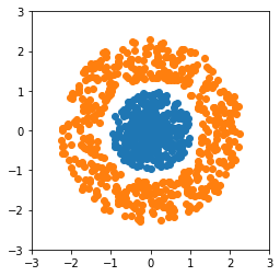
In Figure 1, we can clearly classify the points into blue or orange. Anything that is within then circle of radius 1 is going to be blue and those outside it are likely to be orange. When we encounter a new point, we can still determine accurately which color it will belong to. Point (1,-2) is likely to be orange in color where (0.5,0.5) is likely to be blue.

When we are trying to train a model to do this classification for us, our objective will be to make sure it learns that plane which separates the two data most efficiently. This is where Support Vector Machines (SVM) come in.

In SVM we define the input data as n-dimensional vectors, where n is the number of features present. Let’s us consider a dataset where we have 2 features. We will represent each data item as a point in 2D plane (similar to figure 1). Now we perform classification by finding a hyperplane (a subspace of dimension n-1) which efficiently separates the classes.

Figure 2. Hyperplane separating two different types of data.

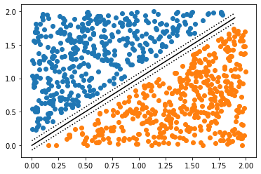
In Figure 2, we can see hyperplanes (lines in this case) separating the two classes of data we have. While the dotted lines are able to separate them correctly, the distance (margin) between them and data points of classes is uneven, it is closer to one class than the other. The continuous line between them however is optimal as the minimum distance between data points of both classes and the separating line is maximum.

SVM identifies such optimal hyperplane which can separate the classes optimally. However will a linear hyperplane be able to separate the distribution in Figure 1? The answer is no, because the distribution is circular in nature and hence requires a circular separator. In this particular case it will be circle with equation x2 + y2 ≈ 1.

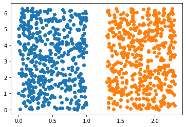
A method to solve such problem can be to represent the data as r and θ, where the angle with respect to x-axis is θ and the radius is r. Using such representation we can separate the data using a linear separation (as shown in Figure 3). Such transformation of data items to aid the classification is defined by kernels associated with the SVM.

Figure 3. Fig 1 represented in linear format.

Let us now try to implement the SVM for binary data classification.

First we need to import the libraries. In this particular scenario we need pandas to import the dataset, numpy for array manipulation and SVM from sklearn for the model.

import pandas as pd
from sklearn import svm
import numpy as np

Next up we will load the dataset in the file “data.csv”

df = pd.read_csv("data.csv",index_col="Index")
print(df.head())

Now we will convert the columns into numpy arrays.

X_value = np.array(df.X).reshape((1000,1))
Y_value = np.array(df.Y).reshape((1000,1))
Labels = np.array(df.Label)
print("X array shape:",X_value.shape)
print("Y array shape:",Y_value.shape)
print("Labels array shape:",Labels.shape)

For SVM, we need to stack the X and Y horizontally in the format [(x1,y1),(x2,y2) ….]. We will do this using hstack function of numpy.

XY = np.hstack([X_value,Y_value])
print("XY array shape:",XY.shape)

Let us now split our dataset into train and test. We will have 80% of the dataset for train while the rest will be for testing.

from sklearn.model_selection import train_test_split
X_train, X_test, y_train, y_test = train_test_split(XY, Labels, test_size=0.2, random_state=2)

Let us now create a Support Vector Classifier for our dataset. We will check the accuracy of our model with respect to the performance on test dataset. By default it considers rbf kernel which is well suited for our dataset as the separation is circular in nature.

clf = svm.SVC()
clf.fit(X_train, y_train)
y_pred = clf.predict(X_test)
from sklearn.metrics import plot_confusion_matrix
plot_confusion_matrix(clf, X_test,y_test)

We can see that the model has about 100% accuracy. This is because both the classes are well separated however while dealing with real dataset the separation between then needn’t be well defined.

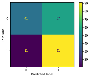
In the below code we see how accurate a SVM with linear kernel. As the the data items cannot be separated using a line, the accuracy is low.

clf = svm.SVC(kernel="linear")
clf.fit(X_train, y_train)
y_pred = clf.predict(X_test)
from sklearn.metrics import plot_confusion_matrix
plot_confusion_matrix(clf, X_test,y_test)

Figure 4. Confusion Matrix for linear classifier.

In this post we have discussed the basics of Support Vector Machines, and how they can be used for binary classification for data. This method has been used in various domains, like sentiment analysis, image classification etc. You can find the code for this blogpost in this github repo.